Model Description
Aevol is a forward-in-time evolutionary simulator that simulates the evolution of a population of organisms through a process of variation and selection. Each artificial organism has an explicit genome, on which RNAs and genes can be identified. The design of the model focuses on the realism of the genome structure and of the mutational process: the mutations affect directly the sequence, without any a priori fitness effect. Aevol can therefore be used to decipher the effect of different operators or processes on genome evolution.
Aevol exists in three flavors: Standard, Eukaryote and 4-Bases. The first two use a binary genomic sequence while the third uses an ATGC-based sequence. Most of the model is identical among the different flavors, and variations will be presented explicitly throughout the model presentation. In short:
- In Standard Aevol, each organism is asexual, haploid, and owns a single circular chromosome. This is inspired by prokaryotic organisms. The genome is encoded as a double-strand binary string. This is the version that has historically been used for most experiments with Aevol (\textit{e.g.} \cite{knibbe2007long,liard2020complexity,banse2023forward}).
- In Eukaryote Aevol, each organism owns two linear chromosomes, and the reproduction is sexual and includes a meiotic recombination event. The genome is encoded as a double-strand binary string.
- In 4-Bases Aevol, the genome is not binary but encoded with the 4 letters ATGC. This changes the genotype-to-phenotype map, but not the rest of the model. It has been used in Liard et al. 2017 and Daudey et al. 2024.
Note that although the Eukaryote and 4-Bases versions could possibly work together, this has not been sufficiently tested yet, and no executable file are generated for the current version of the code.
In Aevol, each individual owns an explicit DNA sequence, composed of 0s and 1s for Standard and Eukaryote Aevol, and ATGCs in 4-Bases Aevol. Genomes are double-stranded, with complementary bases on each strand. Leading and Lagging strands are read in opposite directions.
On the sequence, promoters can be found by pattern recognition based on a consensus sequence. A promoter marks the start of an mRNA. The activity of a promoter is inversely proportional to its distance to the consensus sequence and determines the level of expression of all the protein-coding genes located on the corresponding mRNA. Various conflict resolution strategies are available to handle cases where one gene is present on several mRNAs (for more details, see section Transcription-Translation processes). An mRNA ends at the first encountered terminator sequence. Terminators are defined as sequences that would form a stem-loop structure, as the ρ-independent bacterial terminators do.
On each mRNA, another layer of pattern recognition defines potential genes. The translation is initiated by a Shine-Dalgarno-like sequence followed by a Start codon. When this signal is found on an mRNA, the downstream Open-Reading-Frame (ORF) is read until a Stop codon is found. Each codon lying between the initiation and termination signals is translated into an abstract «amino-acid’’ using an artificial genetic code, thus giving rise to the protein’s primary sequence.
Each protein’s primary sequence is then “folded” into a mathematical function defining the protein’s contribution to the phenotype. This phenotypic contribution is defined as a triangular function, with the coordinate on the abscissa representing the functional space (that can be interpreted as traits) and on the ordinate the level of activation. The phenotype of an individual is the sum of all these protein functions.
Upon replication of an individual, mutations can occur in the sequence. They do not have a predefined fitness effect, as they are applied to positions drawn at random in the genome and the new phenotype is computed afterward.
Mutations can be chromosomal rearrangements (inversions, translocations, duplications, or deletions), or local events (point mutations, InDels). Their rates are per-base and are defined for each mutation type separately.
The population follows a Wright-Fisher model: the whole population is replaced at each generation, and individuals compete to populate the next generation. This competition can either be global, or local on a pre-defined neighborhood except in the Eukaryote model that only allows for global selection. Reproduction is asexual in Standard and 4-Bases Aevol while it is sexual in Eukaryote Aevol. In the latter case, there can be selfing at a predefined rate, and there is always one meiotic recombination upon gametes production.
In Aevol, the Genotype-to-Phenotype-to-Fitness map is based on three major steps corresponding to three different realms:
- A transcription-translation step in which the individuals DNA sequences are parsed to identify mRNAs and genes, and then to translate them into primary protein sequences. This step is globally consistent with biological reality, ensuring the realism of the sequences simulated in Aevol (section Transcription-Translation processes).
- A folding-metabolic step that transforms the primary sequence of the proteins into functional parameters (folding) and combine all protein functions to compute the phenotype (metabolism). This step uses an abstract mathematical representation of the biological processes (section Protein function and phenotype computation).
- A fitness computation step. The phenotype of the organism is compared with an optimal phenotype in order to compute the organism’s fitness (section Environment definition and fitness computation).
The Aevol model
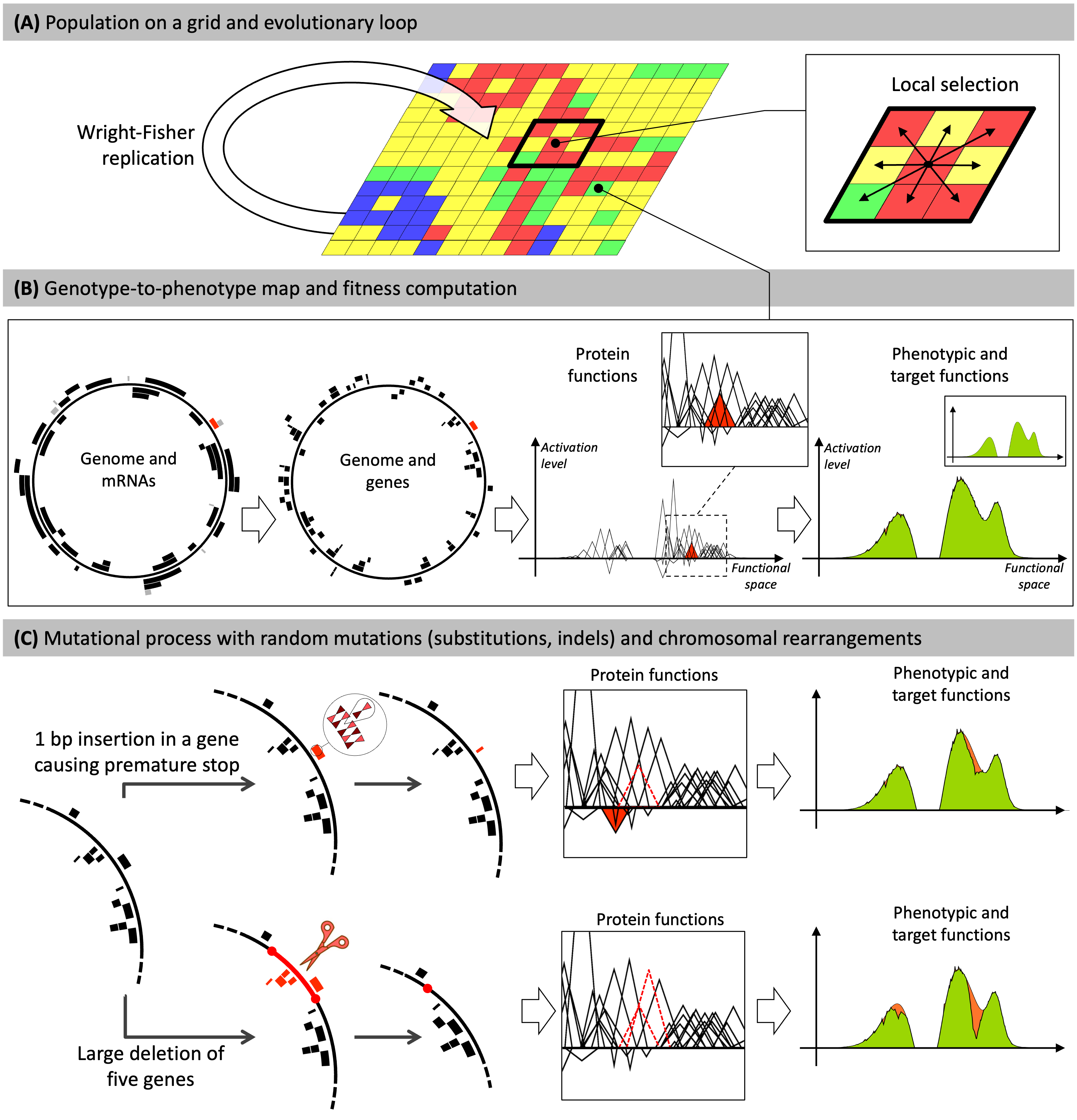
(A) Individuals are distributed on a grid. At each generation, the whole population replicates according to a Wright-Fisher replication model, in which selection operates locally within a \(x \times y\) neighborhood.
(B) Each grid-cell contains a single organism described by its genome. Genomes are decoded through a genotype-to-phenotype map with four main steps (transcription, translation, computation of protein functions, computation of the phenotype). Here, for illustration purposes, a random gene and the corresponding mRNA are colored in red. The red triangle represents the function of this gene in the mathematical world of the model. The phenotypic function is calculated by summing all protein functions. The phenotype is then compared to a predefined target (in green) to compute the fitness. The individual presented here has evolved in the model during \(500,000\) generations.
(C) Individuals may undergo mutations during replication. Two example mutations are shown: a small insertion (top) and a large deletion (bottom).
- Top: A 1 bp insertion occurs within a gene. It causes a frameshift, creating a premature stop codon. The ancestral function of the gene is lost (dashed triangle) and the truncated protein has a deleterious effect (red triangle). This leads to a greater divergence between the phenotype and the target (orange area on the phenotype).
- Bottom: The deletion removes five genes. The functions of two of them can be seen in the box (dotted triangles). This results in a large discrepancy between the phenotype and the target (orange area on the phenotype)
In Aevol each organism owns one (haploid versions) or two (diploid version) DNA sequences. On DNA sequences, mRNAs and genes are delimited by predefined signaling sequences that indicate transcription and translation. The number of proteins an organism has therefore depends on its signaling sequences and can evolve through mutational events.
The Genotype-to-Phenotype-to-Fitness map
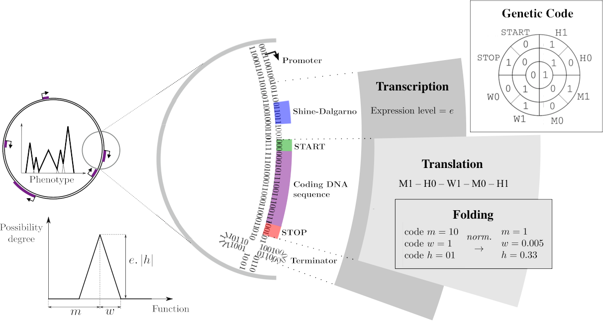
On a DNA sequence, mRNAs are delimited by promoters and terminators, with the expression level resulting from the distance between the promoter and the consensus sequence (Transcription). Within those mRNAs, genes can be identified, starting with a Shine-Darlgarno-Start signal and a Stop codon. Each of these coding sequences is then translated into primary sequences of proteins, using a predefined genetic code (Translation). This primary sequence is decoded as three float parameters called \(m\), \(w\), and \(h\).
Proteins, phenotypes, and environments are represented similarly through mathematical functions that associate a level in \([0, 1]\) to each abstract phenotypic trait in \([0, 1]\). For simplicity reasons, a protein’s contribution is a piecewise-linear function with a triangular shape: the \(m\), \(w\) and \(h\) parameters correspond respectively to the position on the trait space, half-width and height of the triangle. All proteins encoded in the chromosome are then summed to compute the phenotype that, once compared to the environmental target, is be used to compute the fitness of the individual. }
Figure adapted from Daudey et al. 2024.
Transcription starts at promoters, which are defined as sequences that are close enough to an arbitrarily chosen consensus sequence. The expression level \(e\) of an mRNA is determined by the similarity between the actual promoter and the consensus sequence: \(e = 1 - \frac{d}{d_{max} + 1}\) with \(d\) the number of mismatches (\(d\leq d_{max}\)). The consensus sequence is \(0101011001110010010110\) with at most \(d_{max} = 4\) mismatches. This models the interaction of the RNA polymerase with the promoter, without additional regulation.
When a promoter is found, transcription proceeds until a terminator is reached. Terminators are defined as sequences that would form a stem-loop structure, as the ρ-independent bacterial terminators do. The stem size is set to 4 and the loop size to 3. All sequences located between a promoter and a terminator thus correspond to mRNAs in the model.
Once transcribed, mRNAs are then parsed to locate genes and translate them into protein sequences. The translation initiation signal, corresponds to a Shine-Dalgarno-like sequence (aka Ribosome Binding Site – RBS) followed, four bases downstream, by a Start codon. In the Standard and Eukaryote flavours, the Shine-Dalgarno sequence is the six-bp-long sequence \(011011\) and the Start codon is the sequence \(000\) (the full translation initiation signal hence being the sequence \(011011????000\) with \(?\) corresponding to any base).
When this signal is found on an mRNA, the downstream Open-Reading-Frame (ORF) is read codon by codon until a Stop codon is found on the same reading frame (\(001\). An abstract binary genetic code is then used to translate the gene sequence into a protein sequence. In the Standard and Eukaryote flavours, the protein sequence is constructed from a set of 6 Amino-Acids (AA) and the genetic code is an artificial one with no redundancy (Fig. The Genotype-to-Phenotype-to-Fitness map e).
Transcribed sequences (mRNAs) can contain an arbitrary number of ORFs, with some mRNAs possibly containing no ORF at all (non-coding mRNAs) and others possibly containing several ORFs (polycistronic mRNAs). Importantly, the relative fractions of non-coding, monocistronic and polycistronic mRNAs are not predefined but result from the evolutionary dynamics and are likely to be influenced by the evolutionary conditions. Genes can also be nested, or overlapping different reading frames.
Note that in case several promoters are upstream of a translated region, a same gene can be transcribed on several mRNAs. In that case, the expression level of this gene ultimately is equal to the sum of the expression levels of the corresponding mRNAs.
Transcription starts at promoters, which are defined as sequences that are close enough to an arbitrarily chosen consensus sequence. The expression level \(e\) of an mRNA is determined by the similarity between the actual promoter and the consensus sequence: \(e = 1 - \frac{d}{d_{max} + 1}\) with \(d\) the number of mismatches (\(d\leq d_{max}\). In the 4-Bases flavour, that consensus sequence is \(GGCCACCATAGTAGGGTTCATG\) with at most \(d_{max} = 8\) mismatches. In case several promoters are upstream of an RNA, only the farthest promoter is used in the 4-Bases case.
When a promoter is found, transcription proceeds until a terminator is reached. Terminators are defined as sequences that would form a stem-loop structure, as the ρ-independent bacterial terminators do. The stem size is set to 4 and the loop size to 3. All sequences located between a promoter and a terminator thus correspond to mRNAs in the model.
Once transcribed, mRNAs are parsed to locate genes and translate them into protein sequences. The translation initiation signal corresponds to a Shine-Dalgarno-like sequence (a.k.a. Ribosome Binding Site – RBS) followed, four bases downstream, by a Start codon. In the 4-Bases flavour, the Shine-Dalgarno sequence is the six-bp-long sequence \(GATCTC\) and the Start codon is classically the triplet \(ATG\) (the full translation initiation signal hence being the sequence \(GATCTC????ATG\) with \(?\) corresponding to any base).
When this signal is found on an mRNA, the downstream Open-Reading-Frame (ORF) is read one codon at a time until one of the three possible Stop codons is found on the same reading frame (\(TAG\), \(TAA\) or \(TGA\)). The canonical genetic code is then used to translate the gene sequence into the primary protein sequence. Note that, contrary to the Standard and Eukaryote flavours, in the 4-Bases flavour, the genetic code is degenerated and the primary protein sequence is the canonical set of 20 Amino-Acids (AA – see Fig. The genetic code in Aevol 4b). Moreover, in case several promoters are upstream of a translated region, a same gene could be transcribed on several mRNAs. In that case, only the farthest promoter (i.e., only one mRNA is actively transcribing a gene) from the ORF is taken into account to compute the expression level of this gene.
The genetic code in Aevol 4b
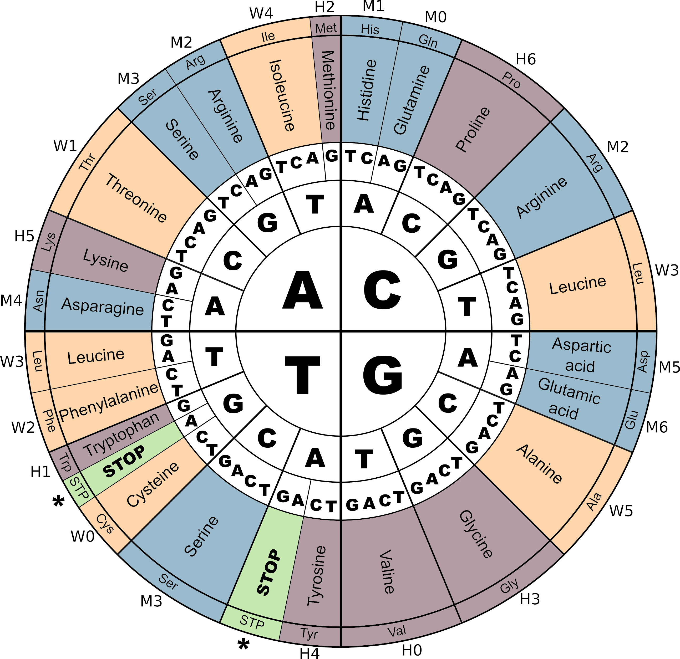
The genetic code and its correspondence with M,W and H digits in Aevol 4b. Notice the three STOP codons (\(TGA\), \(TAG\) and \(TAA\)). As in most biological organisms, the Start codon (\(ATG\)) corresponds to the Amino-Acid Methionine (Met). Colors correspond to the amino-acids contributing to a same parameter (\(m\), \(w\) or \(h\)).
Figure adapted from Daudey et al. 2024.
Transcribed sequences (mRNAs) can contain an arbitrary number of ORFs, with some mRNAs possibly containing no ORF at all (non-coding mRNAs) and others possibly containing several ORFs (polycistronic mRNAs). Importantly, the relative fractions of non-coding, monocistronic and polycistronic mRNAs are not predefined but result from the evolutionary dynamics and are likely to be influenced by the evolutionary conditions. Genes can also be nested or overlap on different reading frames.
At the end of the transcription-translation step, all primary sequences of the organism have been extracted from its genome. The next step consists in computing the functional contribution of each protein and to combine them in order to compute the phenotype of the organism. While in Aevol the transcription-translation process explicitly models the first steps of the central dogma of molecular biology, it would not be possible to model protein functions, metabolism and phenotype with the same accuracy. That is why, in Aevol, we use an abstract representation of the «phenotypic traits» of an organism, that allows fast computation of the function of the proteins and of the phenotype.
We define an abstract continuous one-dimensional space \(\Omega{} = [0,1]\) of phenotypic traits. Each protein is modeled as a mathematical function that associates a contribution level (between \(-1.0\) and \(1.0\)) to a subset of phenotypic traits. For simplicity, we use piecewise-linear functions with a symmetric, triangular shape to model protein effect (Fig. The Genotype-to-Phenotype-to-Fitness map). This way, only three parameters are needed to characterize the contribution of a given protein: the position \(m \in \Omega\) of the triangle on the axis, maximum height \(h\) and its half-width \(w\). In biological terms, \(m\) determines the main function of the protein and \(h\) corresponds to its intrinsic activity (with \(-1\leq h \leq 1\); positive values corresponding to traits activation and negative values corresponding to traits inhibition). Finally, \(w\) sets the range of phenotypic traits to which the protein contributes (pleiotropy). This means that a protein contributes to the phenotypic traits in \([m-w, m+w]\), with a maximal contribution \(h\) for the traits closest to \(m\).
The range of phenotypic traits to which a single protein can contribute is limited by a parameter \(W_{max}\) that sets the maximum pleiotropy degree. Hence, increasing \(W_{max}\) indirectly reduces the total number of proteins required to cover the whole phenotypic space \(\Omega\). Similarly to the \(K\) parameter of the classical \(NK\)-fitness landscape, increasing \(W_{max}\) increases the mean level of pleiotropy and hence the ruggedness of the fitness landscape.
Thus, in Aevol, various types of proteins can exist, from highly efficient (high \(h\)) to poorly efficient (low \(h\)) and even inhibiting (negative \(h\)) and from highly specialized (low \(w\)) to versatile (high \(w\)).
In the Standard and Eukaryote flavours the genome is composed of binary nucleotides. Hence, only 8 different codons are possible, resulting in a simplified genetic code (see Fig The Genotype-to-Phenotype-to-Fitness map and section Transcription-Translation processes) without redundancy and a reduced set of six Amino-Acids (AA): \(M0\), \(M1\), \(H0\), \(H1\), \(W0\) and \(W1\). The primary sequence of a protein is decoded into the three functional parameters \(m\), \(w\) and \(h\) by extracting the three subsequences of \(M0/M1\), \(H0/H1\) and \(W0/W1\) amino-acids and interpreting each subsequence as an integer encoded in binary Gray code (Gray code being used to avoid Hamming cliffs). For instance, the codon \(010\) (resp. \(011\)) is translated into the single amino acid \(W0\) (resp. \(W1\)), which means that it concatenates a bit \(0\) (resp. \(1\)) to the binary code of \(w\). Note that, importantly, the size of the subsequences (hence the length of the binary number) is not predetermined and can evolve (in other words, the gene length is not fixed). A subsequence of length \(L\) can code any integer between \(0\) and \(2^L - 1\). The values of the three parameters are then computed from the decoded integers, normalized depending on their maximum values \(2^L - 1\) and in the range of the corresponding parameter (\([0,1]\) for \(m\), \([-1, 1]\) for \(h\) and \([0,W_{max}]\) for \(w\)).
Mutations in the coding sequences, including local mutations but also chromosomal rearrangements, can change the sequence of codons, hence the subsequences of amino-acids and, ultimately, the protein’s contribution to the phenotype. Note that in particular, mutations can change the length of the proteins, in which case the normalization process will increase the precision of the \(m\), \(h\) and \(w\) values. For instance, a subsequence composed of two \(M\) codons can only encode four values for the \(m\) parameter (\(0\), \(0.33333\), \(0.66666\) and \(1\)) while a subsequence composed of four \(M\) codons can encode 16 different values (\(0\), \(0.06667\), \(0.12222\), \(…\) , \(0.93333\) and \(1\)). In other words, increasing the length of the genes allows the accuracy of the proteins function to increase.
Contrary to the Standard and Eukaryote flavours that use binary nucleotides, the 4-Bases flavour uses a 4-base nucleotide alphabet decoded using the canonical degenerated genetic code (see Fig The genetic code in Aevol 4b). Hence, the primary sequence of a protein is composed of an arbitrary number of amino-acids (AA). To decode it into the three functional parameters \(m\), \(w\) and \(h\), we first associate each AA to one of the parameters, with a weighted contribution, between \(0\) and \(6\) for \(m\) and \(h\) and between \(0\) and \(5\) for \(w\) – see Fig The genetic code in Aevol 4b, external circle. Note that this repartition has been randomly generated and has no explicit biological meaning.
We then extract the three subsequences of all AAs associated with \(m\), \(w\) and \(h\) respectively. Given the weights of the different AAs in these three subsequences, we compute an integer value for each of them (through the decoding of a modular Gray code in base \(7\) for \(m\) and \(h\) and in base \(6\) for \(w\) – Gray code being used to avoid Hamming cliffs). For instance, the sequence \(TCC–CAT–CGG\) is translated into a Serine followed by an Histidine and an Arginine, hence into an \(M3\) followed by an \(M1\) and an \(M2\) (giving the value 312 in base 7 Gray encoding), which results in the integer value 181 (in decimal encoding).
Importantly, the size of the subsequences is not predetermined and can evolve (in other words, the gene length is not fixed). A subsequence of length \(L\) can code any integer between \(0\) and \(7^L - 1\) (for \(m\) and \(h\)) and between \(0\) and \(6^L - 1\) (for \(w\)) . The values of the three parameters are then computed from the decoded integers, normalized depending on their maximum values and in the range of the corresponding parameter (\([0,1]\) for \(m\), \([-1, 1]\) for \(h\) and \([0,W_{max}]\) for \(w\)). For instance, the sequence \(TCC–CAT–CGG\) presented above would result in an \(m\) value equal to \(m = 181/(7^3 - 1) = 181/342 = 0.529240\).
Mutations in the coding sequences, including local mutations but also chromosomal rearrangements, can change the sequence of codons, hence the subsequences of amino-acids and, ultimately, the protein’s contribution to the phenotype. In particular, mutations can change the length of proteins, in which case the normalization process will increase the precision of the \(m\), \(h\) and \(w\) values. For instance, a subsequence composed of a single \(M\) codon can encode seven values for the \(m\) parameter (\(0\), \(0.16667\), \(0.33333\), \(0.5\), \(0.66667\), \(0.83333\) and \(1\)) while a subsequence composed of two \(M\) codons can encode \(7^2 = 49\) different values (\(0\), \(0.02083\), \(0.04166\), \(…\) , \(0.97917\), \(1\)). In other words, increasing the length of the genes allows the accuracy of the proteins function to increase.
For all three flavours of Aevol, once the protein functions have been computed, the contribution of all the proteins encoded in the genotype of an organism are combined to get the final level for each phenotypic trait. This is done by first scaling all protein contributions by the transcription rate \(e\) of the corresponding mRNA(s) (see above), then by summing independently the mathematical functions of all the proteins activating phenotypic traits (i.e. proteins for which \(h > 0\)) and for proteins inhibiting phenotypic traits (i.e. proteins for which \(h < 0\)), with bounds in \(0\) and \(\pm 1\). The final level of each phenotypic trait is then obtained by subtracting the inhibited traits to the activated ones, with a 0 bound. Formally this procedure corresponds to combining sets of activated/inhibited traits using Lukasiewicz operations, a trait being activated if it is activated by the set of activating proteins and not inhibited by the set of inhibiting proteins. The resulting piecewise-linear function \(P: \Omega{} \rightarrow [0, 1]\) is called the phenotype of the organism (see Figure The Aevol model B).
Note that, in the Eukaryote case, all proteins from both chromosomes are treated identically and summed together.
The environment is defined as a target activation level for each trait, i.e. a mathematical function \(E: \Omega{} \rightarrow [0, 1]\) (see above). This target function indicates the optimal level of each phenotypic trait in \(\Omega{}\) and is called the environmental target. \(E\) is classically defined as the sum of several Gaussian lobes, which standard deviations, maximal heights and centers are set by the user at the start of the simulation.
In the model, fitness depends only on the difference between the levels of the phenotypic traits and the environmental target.
The difference between \(P\) and \(E\) is defined as \(\Delta:=\int_\Omega{}|E(x) - P(x)| dx, \forall x\in\Omega\) and is called the «metabolic error». It is used to measure adaptation penalizing both the under-realization and the over-realization of phenotypic traits. Given the metabolic error of an individual, its fitness \(f\) is given by \(f:=\exp(-k \Delta)\) with \(k\) a fixed parameter regulating the selection strength (the higher \(k\), the larger the effect of metabolic error variations on the fitness values).
The population is modelled as a toroidal grid with one individual per grid cell. At each generation, the fitness of each individual is computed, and the individuals compete to populate each cell of the grid at the next generation. This competition can be fully local (the 9 individuals in the neighborhood of a given cell competing to populate it at the next generation, Fig. The Aevol model A) or encompass a larger subpopulation. If the selection scope encompasses the whole population, all individuals compete for all grid cells.
Importantly, the more local the selection scope, the more the population model diverges from the panmictic Wright-Fisher model as local selection increases the effective population size \(N_e\) for a given census population size. Given a selection scope, the individuals in the neighborhood \(\mathcal{N}\) of a given grid-cell compete through a «fitness-proportionate» selection scheme: the probability \(p_j\), for an individual \(j\) with fitness \(f_j\) to populate the focal grid-cell at the next generation is given by \(p_j=f_j/\sum_{i\in \mathcal{N}} f_i\).
In the Eukaryote case, two parents are needed for the reproduction. If no constrain on the selfing proportion is set, the two parents are drawn with the above-described process, and they can be the same individual or be different. If a selfing proportion \(p\) is set by the user, there is a \(p\) chance to draw just one parent and use it as second parent two, and a \(1 - p\) chance to force the draw of two different parent (parent1 is removed from the pool of possible parents for parent2).
During their replication, genomes can undergo sequence variations (Fig. The Aevol model D). An important feature of the model is that, given the Genotype-to-Phenotype map, any genome sequence can be decoded into a phenotype (although possibly with no trait activated if there is no ORF on the sequence). This allows implementation – and testing – of any kind of mutational process. In the classical usage of the simulator, seven different kinds of mutations are modeled (depicted on Fig. Mutation operators in Aevol).
The rates \(mu_{t}\) at which each type \(t\) of genetic mutation occur are defined as a per-base, per-replication probability, and so the number of spontaneous events is linearly dependent on the length of the genome. However, their fixation probability depends on their phenotypic effect (for instance, a mutation affecting exclusively an untranscribed region is likely to be neutral). Hence, the distribution of fitness effects (DFE) of any kind of mutation is not predefined but depends on the intertwining of its effect on the sequence, and of the genome structure. For example, the fraction of coding sequences or the spatial distribution of the genes along the chromosome change the probability of a given mutation to alter the phenotype, and the fitness, an effect that is especially important for chromosomal rearrangements. Having an emergent DFE instead of a predefined one enables investigating the complex direct and indirect effects of chromosomal rearrangements on the evolutionary dynamics.
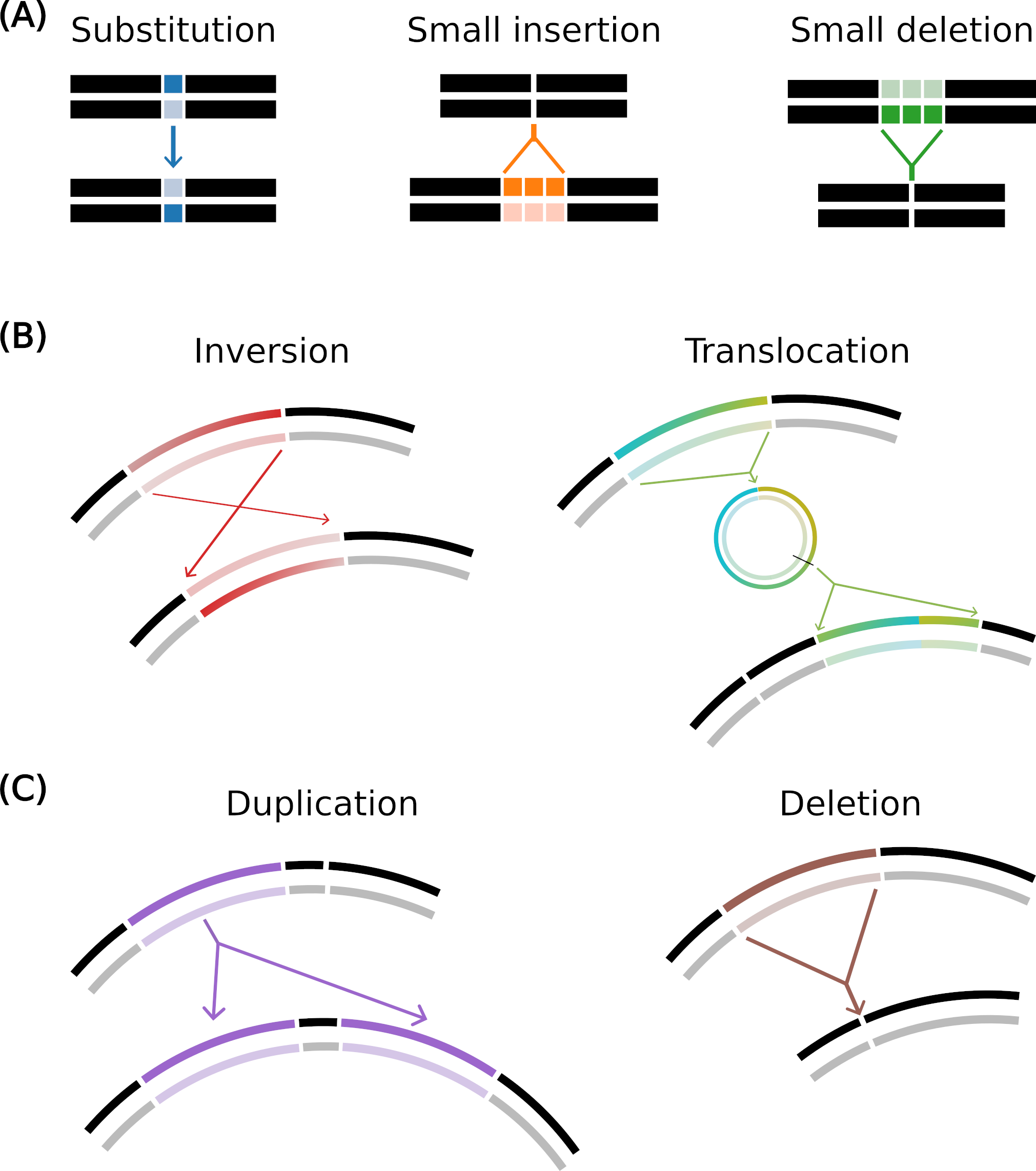
Mutation operators in Aevol
(A) Local mutations: substitution (one base pair is mutated to another), small insertion and small deletion (a few base pairs are inserted or deleted).
(B) Balanced chromosomal rearrangements: inversion (two points are drawn and the segment in between is rotated) and translocation (a segment is excised, circularized, re-cut and inserted elsewhere in the genome).
(C) Unbalanced chromosomal rearrangements: duplication (copy-paste of a segment in the genome) and deletion (suppression of a segment of the genome).
There are three types of local mutations : substitution, small insertion and small deletion. They happen at a position uniformly drawn on the genome. Substitutions change a single nucleotide to any of the other possible ones (\(0\) to \(1\) or \(1\) to \(0\) in the Standard and Eukaryote, and with a uniform probability to any of the three other letters in 4-Bases).
InDels insert (or delete) a small sequence of random length – and random composition for insertions. The length of the sequence is drawn uniformly between 1 and a maximum value (6 by default). Notably, InDels occurring within an ORF can shift the reading frame or simply add/remove codons, resulting in very different evolutionary outcomes.
There are four types of chromosomal rearrangements: translocations and inversions (which are balanced, i.e. they don’t change the genome length), and duplications and deletions (which are unbalanced). Note that in the Eukaryote flavor of Aevol, translocations can only happen within one chromosome and not between them.
Chromosomal rearrangement breakpoints are uniformly drawn on the chromosome, the number of breakpoints depending on the type of rearrangement (Fig. Mutation operators in Aevol). Hence, chromosomal rearrangements can be of any size between 1 and the total genome size, allowing to investigate the effect of structural variants that are indeed observed in vivo.
In the Standard and 4-Bases cases, the positions drawn are ordered (\(p1\) and \(p2\)) and the segment of interest – which will be duplicated/deleted/inverted/translocated – is from \(p1\) to \(p2\), and possibly go over the position \(0\) as the chromosome is circular.
In the Eukaryote case however, the segment of interest cannot go over the position \(0\) as chromosome are linear, and we invert \(p1\) and \(p2\) if necessary. Also note that chromosomal rearrangements are confined to a single chromosome: segments are only duplicated or translocated within a chromosome.
As they can change the structure of the genome, chromosomal rearrangements are applied first, before the local mutation events.
This section is only relevant to the Eukaryote flavor of Aevol. Each parent transmits a recombined chromosome to its children. To perform a recombination, an alignment between the two parental chromosomes is searched, and the alignment point is used as a breaking point to recombine the two chromosomes (see Fig Meiotic recombination). Then, one of the two recombined chromosomes is transmitted to the offspring (and will undergo rearrangements and local mutations). Note that the process occurs at each reproduction event: a parent having \(n\) offspring will make at least \(n\) different recombinations, and an individual chosen twice as parent of the same individual (selfing) will make two different recombinations for this offspring.
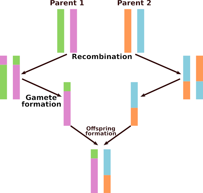
Meiotic recombination
Meiotic recombination in the Eukaryote flavor of Aevol.
To perform an evolutionary experiment with Aevol, the population and environment must first be initialised with aevol_create. Then, aevol_run is used to simulate a certain number of generations forward-in-time.
In the Standard and 4-Bases flavors, it is also possible to recreate a lineage of unique ancestors starting from the final population (aevol_post_lineage), and to perform analyses on that lineage instead of on the whole population. Generally, the stats on the lineage of the population (ancestors stats) is analysed as the description of the evolution, using aevol_post_ancestor_stats.
More details about the how to install Aevol and how to use it are provided in the Installation and User Documentation pages.
During the simulation, everything is known about each individual and replication event. Not all information can be recorded as it would take too much space on the disk, but there are several options to record relevant information.
Stats on the best individual of the population can be recorded at a given frequency (STATS_BEST keyword in parameter file).
The mean value for the population for these stats can also be recorded (STATS_POP keyword in parameter file). However, we recommend recording these values at a lower frequency to avoid unnecessary computational costs.
These stats provide information on the dynamics of evolution, and especially on the evolution of genome structure, which is highly variable.
Content of a stat file describing an individual (best individual or ancestor individual of the population).
| Name in the stats file | Description |
|---|---|
| Generation | Generation of the individual of interest |
| pop_size | Population size |
| indiv_idx | Index of the individual of interest |
| fitness | Fitness of the individual of interest |
| metabolic_error | Metablic error of the individual of interest. The metabolic error is the distance between the individual’s phenotype and the environmental target |
| amount_of_dna | Number of base pairs of the individual of interest |
| nb_coding_rnas | Number of coding RNAs of the individual of interest |
| av_len_coding_rnas | Average length (in base pairs) of the coding RNAs of the individual of interest |
| nb_non_coding_rnas | Number of non-coding RNAs of the individual of interest |
| nb_functional_genes | Number of functional genes of the individual of interest |
| av_len_functional_genes | Average length (in base pairs) of the functional genes of the individual of interest |
| nb_non_functional_genes | Number of non-functional genes of the individual of interest |
| nb_mut | Number of mutation undergone by the individual of interest at its birth |
| nb_switch | Number of switch undergone by the individual of interest at its birth |
| nb_indels | Number of indels undergone by the individual of interest at its birth. Indels are small insertions or small deletions |
| nb_rear | Number of chromosomal rearrangements undergone by the individual of interest at its birth |
| nb_dupl | Number of duplications undergone by the individual of interest at its birth |
| nb_del | Number of deletions undergone by the individual of interest at its birth |
| nb_trans | Number of translocations undergone by the individual of interest at its birth |
| nb_inv | Number of inversions undergone by the individual of interest at its birth |
| non_coding_bp | Number of non-coding base pairs of the individual of interest (only in ancestor stats file on in Eukaryote flavour) |
| Name in the stats file | Description |
|---|---|
| Generation | Generation of the population |
| pop_size | Population size |
| fitness | Average fitness of the population |
| metabolic_error | Average metabolic error of the population. The metabolic error is the distance between an individual’s phenotype and the environmental target |
| amount_of_dna | Average number of base pairs of the individuals in the population |
| nb_coding_rnas | Average number of coding RNAs of the individuals in the population |
| av_len_coding_rnas | Average of the average lengths (in base pairs) of coding RNAs of the individuals in the population |
| nb_non_coding_rnas | Average number of non-coding RNAs of the individuals in the population |
| nb_functional_genes | Average number of functional genes of the individuals in the population |
| av_len_functional_genes | Average of the average lengths (in base pairs) of the functional genes of the individuals in the population |
| nb_non_functional_genes | Average number of non-functional genes of the individuals in the population |
| non_coding_bp | Average number of non-coding bases of the individuals in the population |
| selfing_rate | Measured selfing rate for the population at this generation (Eukaryote only) |
As simulations can be very long, Aevol outputs regular checkpoints that allow resuming the simulation at a specific generation instead of having to restart it.
A checkpoint consists of 3 files: a population file containing the genome sequences of all the individuals in the population in fasta format, a setup file containing general setup parameters that can be modified, and a semi-opaque checkpoint file containing object states
Relevant information on each replication event can also be recorded: the parent/offspring relationships and all the mutation events of each replication are stored in the «Trees».
This data structure is not readable by other programs, but several Aevol programs for post-evolution analyses can open it to extract data of interest. Most importantly, Trees are used by aevol_post_lineage to reconstruct the lineage of an individual of the final population.
Having the perfect knowledge of everything that happened during the evolution, it is possible to dig further into the experiments to study specific evolutionary behaviors. Additional post-treatments of the data can be developed for specific needs of each evolutionary experiment performed with Aevol, but we present here those that were most recently used. Further details on their usage is presented in the User Documentation page.
Aevol allows for the extraction of specific individuals who lived during a simulation (on the lineage of the final population or any arbitrary individual) and the performing of mutations on them to observe their response. For substitutions, it is possible to test every possible mutation and observe its effect on the fitness of the individual. For other, more complex types of mutations, it is possible to perform an arbitrary number of mutations to extract experimentally their distribution of fitness effects.
Aevol allows extracting specific individuals that lived during a simulation (on the lineage of the final population, or any arbitrary individual) and performing replications on them to observe their response.
By performing a high number of different replications from one individual, we can experimentally compute its replicative robustness (probability that a replication is neutral in terms of fitness), as well as its evolvability (defined as the proportion of beneficial mutations multiplied by their average gain in fitness).
- Vincent Liard, Jonathan Rouzaud-Cornabas, Nicolas Comte, Guillaume Beslon (2017). A 4-base model for the Aevol in-silico experimental evolution platform. Proceedings of ECAL 2017, the Fourteenth European Conference on Artificial Life.
- Hugo Daudey, David P. Parsons, Eric Tannier, Vincent Daubin, Bastien Boussau, Vincent Liard, Romain Gallé, Jonathan Rouzaud-Cornabas, Guillaume Beslon (2024). Aevol_4b: Bridging the gap between artificial life and bioinformatics. Proceedings of the 2024 Artificial Life Conference.